
The State of Observability
Realize 2.67x returns on investments. See how in our latest State of Observability report.

The stats, chart, and timechart commands are great commands to know (especially stats). When I first started learning about the Splunk search commands, I found it challenging to understand the benefits of each command, especially how the BY clause impacts the output of a search. It wasn't until I did a comparison of the output (with some trial and a whole lotta error) that I was able to understand the differences between the commands.
These three commands are transforming commands. A transforming command takes your event data and converts it into an organized results table. You can use these three commands to calculate statistics, such as count, sum, and average.
Note: The BY keyword is shown in these examples and in the Splunk documentation in uppercase for readability. You can use uppercase or lowercase in your searches when you specify the BY keyword.
Let's start with the stats command. We are going to count the number of events for each HTTP status code.
... | stats count BY status
The count of the events for each unique status code is listed in separate rows in a table on the Statistics tab:
| status | count |
|---|---|
| 200 | 34282 |
| 400 | 701 |
| 403 | 228 |
| 404 | 690 |
Basically the field values (200, 400, 403, 404) become row labels in the results table.
For the stats command, fields that you specify in the BY clause group the results based on those fields. For example, we receive events from three different hosts: www1, www2, and www3. If we add the host field to our BY clause, the results are broken out into more distinct groups.
... | stats count BY status, host
Each unique combination of status and host is listed on a separate row in the results table.
| status | host | count |
|---|---|---|
| 200 | www1 | 11835 |
| 200 | www2 | 11186 |
| 200 | www3 | 11261 |
| 400 | www1 | 233 |
| 400 | www2 | 257 |
| 400 | www3 | 211 |
| 403 | www2 | 228 |
| 404 | www1 | 244 |
| 404 | www2 | 209 |
| 404 | www3 | 237 |
Each field you specify in the BY clause becomes a separate column in the results table. You're splitting the rows first on status, then on host. The fields that you specify in the BY clause of the stats command are referred to as <row-split> fields.
In this example, there are five actions that customers can take on our website: addtocart, changequantity, purchase, remove, and view.
Let's add action to the search.
... | stats count BY status, host, action
You are splitting the rows first on status, then on host, and then on action. Below is a partial list of the results table that is produced when we add the action field to the BY clause:
| status | host | action | count |
|---|---|---|---|
| 200 | www1 | addtocart | 1837 |
| 200 | www1 | changequantity | 428 |
| 200 | www1 | purchase | 1860 |
| 200 | www1 | remove | 432 |
| 200 | www1 | view | 1523 |
| 200 | www2 | addtocart | 1743 |
| 200 | www2 | changequantity | 365 |
| 200 | www2 | purchase | 1742 |
One big advantage of using the stats command is that you can specify more than two fields in the BY clause and create results tables that show very granular statistical calculations.
Using the same basic search, let's compare the results produced by the chart command with the results produced by the stats command.
If you specify only one BY field, the results from the stats and chart commands are identical. Using the chart command in the search with two BY fields is where you really see differences.
Remember the results returned when we used the stats command with two BY fields are:
| status | host | count |
|---|---|---|
| 200 | www1 | 11835 |
| 200 | www2 | 11186 |
| 200 | www3 | 11261 |
| 400 | www1 | 233 |
| 400 | www2 | 257 |
| 400 | www3 | 211 |
| 403 | www2 | 228 |
| 404 | www1 | 244 |
| 404 | www2 | 209 |
| 404 | www3 | 237 |
Now let's substitute the chart command for the stats command in the search.
... | chart count BY status, host
The search returns the following results:
| status | www1 | www2 | www3 |
|---|---|---|---|
| 200 | 11835 | 11186 | 11261 |
| 400 | 233 | 257 | 211 |
| 403 | 0 | 288 | 0 |
| 404 | 244 | 209 | 237 |
The chart command uses the first BY field, status, to group the results. For each unique value in the status field, the results appear on a separate row. This first BY field is referred to as the <row-split> field. The chart command uses the second BY field, host, to split the results into separate columns. This second BY field is referred to as the <column-split> field. The values for the host field become the column labels.
Notice the results for the 403 status code in both results tables. With the stats command, there are no results for the 403 status code and the www1 and www3 hosts. With the chart command, when there are no events for the <column-split> field that contain the value for the <row-split> field, a 0 is returned.
One important difference between the stats and chart commands is how many fields you can specify in the BY clause.
With the stats command, you can specify a list of fields in the BY clause, all of which are <row-split> fields. The syntax for the stats command BY clause is:
BY <field-list>
For the chart command, you can specify at most two fields. One <row-split> field and one <column-split> field.
The chart command provides two alternative ways to specify these fields in the BY clause. For example:
... | chart count BY status, host
... | chart count OVER status BY host
The syntax for the chart command BY clause is:
[ BY <row-split> <column-split> ] | [ OVER <row-split> ] [BY <column-split>] ]
The advantage of using the chart command is that it creates a consolidated results table that is better for creating charts. Let me show you what I mean.
When you run the stats and chart commands, the event data is transformed into results tables that appear on the Statistics tab. Click the Visualization tab to generate a graph from the results. Here is the visualization for the stats command results table:
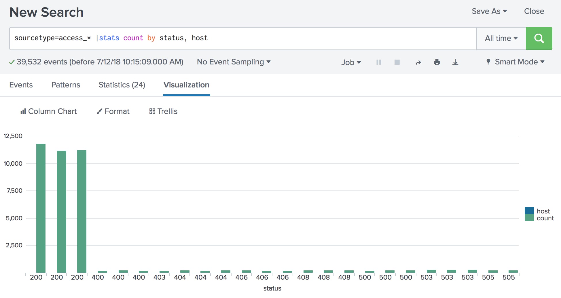
The status field forms the X-axis, and the host and count fields form the data series. The range of count values form the Y-axis.
There are several problems with this chart:
Because of these issues, the chart is confusing and does not convey the information that is in the results table.
While you can create a usable visualization from the stats command results table, the visualization is useful only when you specify one BY clause field.
It's better to use the chart command when you want to create a visualization using two BY clause fields:
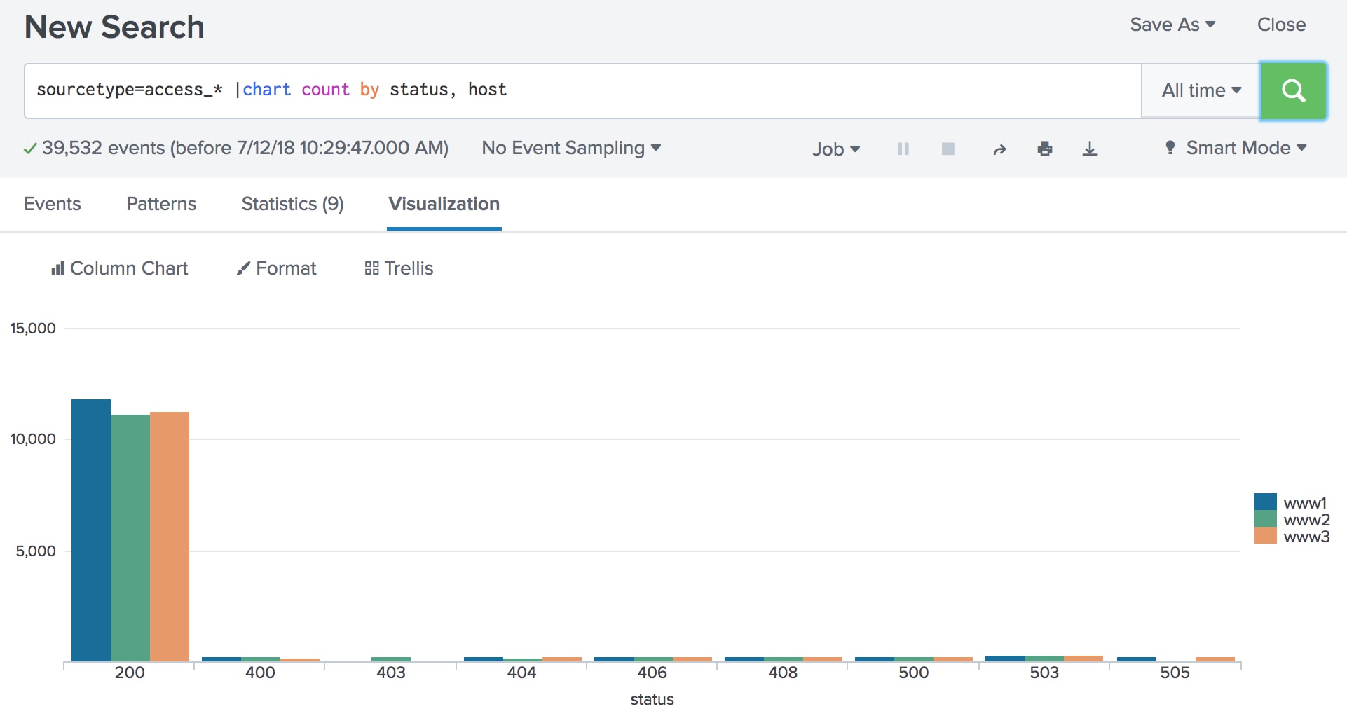
The status field forms the X-axis and the host values form the data series. The range of count values form the Y-axis.
When you use the timechart command, the results table is always grouped by the event timestamp (the _time field). The time value is the <row-split> for the results table. So in the BY clause, you specify only one field, the <column-split> field. For example, this search generates a count and specifies the status field as the <column-split> field:
... | timechart count BY status
This search produces this results table:
| _time | 200 | 400 | 403 | 404 |
|---|---|---|---|---|
| 2018-07-05 | 1038 | 27 | 7 | 19 |
| 2018-07-06 | 4981 | 111 | 35 | 98 |
| 2018-07-07 | 5123 | 99 | 45 | 105 |
| 2018-07-08 | 5016 | 112 | 22 | 105 |
| 2018-07-09 | 4732 | 86 | 34 | 84 |
| 2018-07-10 | 4791 | 102 | 23 | 107 |
| 2018-07-11 | 4783 | 85 | 39 | 98 |
| 2018-07-12 | 3818 | 79 | 23 | 74 |
If you search by the host field instead, this results table is produced:
_time | www1 | www2 | www3 |
|---|---|---|---|
| 2018-07-05 | 372 | 429 | 419 |
| 2018-07-06 | 2111 | 1837 | 1836 |
| 2018-07-07 | 1887 | 2046 | 1935 |
| 2018-07-08 | 1927 | 1869 | 2005 |
| 2018-07-09 | 1937 | 1654 | 1792 |
| 2018-07-10 | 1980 | 1832 | 1733 |
| 2018-07-11 | 1855 | 1847 | 1836 |
| 2018-07-12 | 1559 | 1398 | 1436 |
The time increments that you see in the _time column are based on the search time range or the arguments that you specify with the timechart command. In the previous examples the time range was set to All time and there are only a few weeks of data. Because we didn't specify a span, a default time span is used. In this situation, the default span is 1 day.
If you specify a time range like Last 24 hours, the default time span is 30 minutes. The Usage section in the timechart documentation specifies the default time spans for the most common time ranges. This results table shows the default time span of 30 minutes:
| _time | www1 | www2 | www3 |
|---|---|---|---|
| 2018-07-12 15:00:00 | 44 | 22 | 73 |
| 2018-07-12 15:30:00 | 34 | 53 | 31 |
| 2018-07-12 16:00:00 | 14 | 33 | 36 |
| 2018-07-12 16:30:00 | 46 | 21 | 54 |
| 2018-07-12 17:00:00 | 75 | 26 | 38 |
| 2018-07-12 17:30:00 | 38 | 51 | 14 |
| 2018-07-12 18:00:00 | 62 | 24 | 15 |
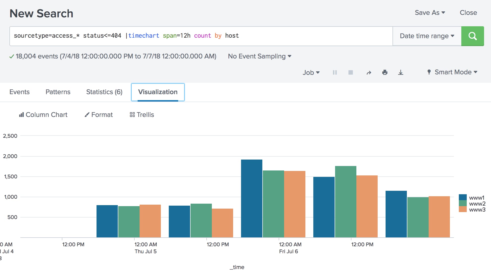
The timechart command includes several options that are not available with the stats and chart commands. For example, you can specify a time span like we have in this search:
... | timechart span=12h count BY host
| _time | www1 | www2 | www3 |
|---|---|---|---|
| 2018-07-04 17:00 | 801 | 783 | 819 |
| 2018-07-05 05:00 | 795 | 847 | 723 |
| 2018-07-05 17:00 | 1926 | 1661 | 1642 |
| 2018-07-06 05:00 | 1501 | 1774 | 1542 |
| 2018-07-06 17:00 | 2033 | 1909 | 1857 |
| 2018-07-07 05:00 | 1482 | 1671 | 1594 |
| 2018-07-07 17:00 | 2027 | 1818 | 2036 |
In this example, the 12-hour increments in the results table are based on when you run the search (local time) and how that aligns that with UNIX time (sometimes referred to as epoch time).
Note: There are other options you can specify with the timechart command, which we'll explore in a separate blog.
So how do these results appear in a chart? On the Visualization tab, you see that _time forms the X-axis. The axis marks the Midnight and Noon values for each date. However, the columns that represent the data start at 1700 each day and end at 0500 the next day.
The field specified in the BY clause forms the data series. The range of count values forms the Y-axis.
The stats, chart, and timechart commands have some similarities, but you’ve got to pay attention to the BY clauses that you use with them.
Other blogs:
Splunk documentation:

The world’s leading organizations rely on Splunk, a Cisco company, to continuously strengthen digital resilience with our unified security and observability platform, powered by industry-leading AI.
Our customers trust Splunk’s award-winning security and observability solutions to secure and improve the reliability of their complex digital environments, at any scale.

Get the latest articles from Splunk straight to your inbox.
© 2005 - 2025 Splunk LLC All rights reserved.