Causal Inference: Determining Influence in Messy Data

When analysing data one of the biggest questions you may often face is: what is causing this situation? In this blog, we’re going to look at how causal inference can be used to understand in more detail what the biggest influencing factors are across a dataset. 

Traditionally in Splunk, we talk about correlation; does metric x go up or down in accordance with metric y or is there a relationship between x and y?

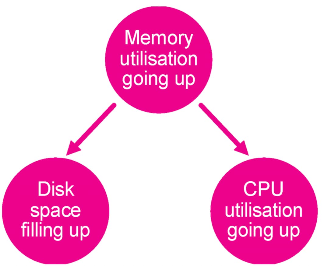
This has flaws of course, as you could assume that correlation equals causation – for example that CPU going up is a direct result of the disk space filling up, where in fact they are both caused by the memory utilisation going through the roof. 

So, what can we do to help identify these causal relationships in data? Here we are going to use the Deep Learning Toolkit, SMLE and a python library designed to identify causal relationships in data. There are a number of libraries out there to choose from, but here we have gone for the CausalNex library put together by some of the awesome folks at QuantumBlack Labs.

Directional Acyclic Graphs

The CausalNex library focuses on using directional acyclic graphs (DAGs), which are useful data structures that share a lot of similarities with traditional graph analytics. The main difference between the types of graphs analysed in previous apps and blogposts and DAGs is that a DAG contains more information about the direction of the relationship between two nodes. This is illustrated in the basic example using memory utilisation above, but we’re going to explore it in more detail here. 

There are loads of use cases for DAGs, but one you will (hopefully) be familiar with is a family tree. In our case, we’re going to use them to see if we can understand which data points are having the most impact on the thing we are monitoring or care about the most – so there are some really interesting applications in root cause analysis, which I will talk about more in the future!

Installing CausalNex

To begin with, you will need to install the DLTK and its pre-requisites and also spin up an environment where you have Docker running. There’s a great walkthrough here that you can follow to make all the installs and get a container up and running.

Once you have a version of the DLTK up and running in your Splunk instance we can then pick up with the installation steps for CausalNex. To start off with go to the containers dashboard (under configuration) and spin up a container using the golden image. When this is running we need to find the Docker container that has been initiated by the DLTK, so you need to run this in the shell of the environment you are running Docker in:

docker ps

This will provide you with a list of running containers in the environment. To find the running golden image look for the container that has the image phdrieger/mltk-container-golden-image-gpu:3.3.2 and take a note of its name. We can then connect to the container using the following:

docker exec -it --user="root" <container_name> /bin/bash

Note that we are connecting as the root user to make sure that our installs are visible to Splunk. Once in the container, we run the following to install the CausalNex library:

pip install causalnex

Easy right! 

There are a couple of additional installs we need to make if we want to use the visualisations that come as part of the CausalNex library, which are Pygraphviz, Graphviz and Pydot. To install these in the container we also need to run in order:

apt-get install graphviz

pip install graphviz

pip install pydot

pip install pygraphviz

This is all we need to start writing our code in the DLTK.

Developing the Code

We are going to follow the DAG regressor example in the CausalNex documentation for our notebook. The first thing for us to do is take a copy of the barebone.ipynb notebook and rename it causalnex.ipynb.

For Stage 0 – Import libraries enter the following:

import json
import numpy as np
import pandas as pd
from causalnex.structure import DAGRegressor
from sklearn.model_selection import cross_val_score
from sklearn.preprocessing import StandardScaler
from sklearn.model_selection import KFold

MODEL_DIRECTORY = "/srv/app/model/data/"

We’re not going to do anything with stage 1, though feel free to send some sample data over from Splunk using the mode=stage option in the MLTKContainer fit command to use for experimenting in your notebook. Moving on to Stage 2 we need our model definition code:

def init(df,param):

    model = DAGRegressor(

                alpha=0.1,

                beta=0.9,

                fit_intercept=True,

                hidden_layer_units=None,

                dependent_target=True,

                enforce_dag=True,

                 )

    return model

We are then going to write the code to fit the mode in stage 3, noting that we are applying a scaling algorithm to our data before fitting the DAGRegressor: 

def fit(model,df,param):
    
    target=param['target_variables'][0]
    
    #Data prep for processing
    y_p = df[target]
    y = y_p.values

    X_p = df[param['feature_variables']]
    X = X_p.to_numpy()
    X_col = list(X_p.columns)

    #Scale the data
    ss = StandardScaler()
    X_ss = ss.fit_transform(X)
    y_ss = (y - y.mean()) / y.std()
    
    scores = cross_val_score(model, X_ss, y_ss, cv=KFold(shuffle=True, random_state=42))
    print(f'MEAN R2: {np.mean(scores).mean():.3f}')

    X_pd = pd.DataFrame(X_ss, columns=X_col)
    y_pd = pd.Series(y_ss, name=target)

    model.fit(X_pd, y_pd)
    
    info = pd.Series(model.coef_, index=X_col)
    #info = pd.Series(model.coef_, 
index=list(df.drop(['_time'],axis=1).columns))
    return info

Finally, for stage 4 we need the code to apply our model and generate the results, which looks like:

def apply(model,df,param):
    data = []

    for col in list(df.columns):
        s = model.get_edges_to_node(col)
        for i in s.index:
            data.append([i,col,s[i]]);

    graph = pd.DataFrame(data, columns=['src','dest','weight'])

    #results to send back to Splunk
    graph_output=graph[graph['weight']>0]
    return graph_output

Ultimately this code is taking the DAGRegressor model and turning it into a dataframe that can be returned to our Splunk instance for further analysis and visualisation. 

The last thing to do is to make sure that the final few stages are blank as we are not going to save, reload or summarise the model here.

Causal Inference in Action 

Now that we have our code up and running it is time to see what it does! 

First of all, we’re going to see the type of visualisations that are possible with the CausalNex library within our notebook. Running the search below from Splunk will send our housing data over to our container environment:

| inputlookup housing.csv

| fit MLTKContainer mode=stage algo=causalnex "median_house_value" from *

Once this data is accessible in the /notebooks/data/ folder in the Jupyter lab we can run the following at the end of our notebook to generate the visualisation:

df, param = stage("causalnex")

model = init(df,param)

fit(model,df,param)

apply(model,df,param)

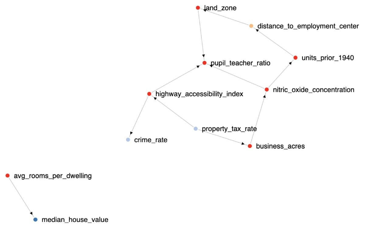
model.plot_dag(True)

We could at this point send the visualisation back to Splunk as shown here, or we could run the fit command to return the data to Splunk for visualisation using the search below:

| inputlookup housing.csv

| fit MLTKContainer algo=causalnex "median_house_value" from *

| rename "predicted_median_house_value" as src

| table dest src weight

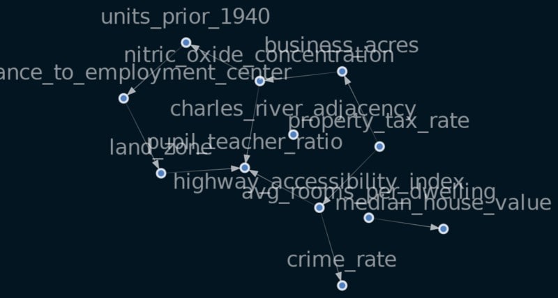
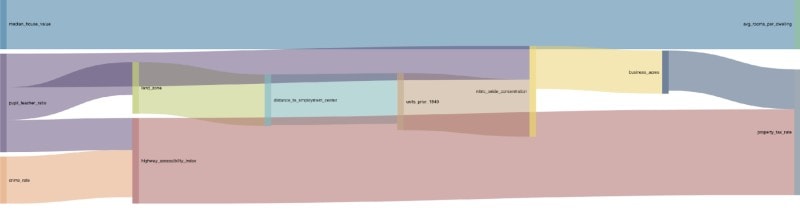
The results of this search can be visualised using the force directed or Sankey diagram to understand which variables have the biggest impact on the others.

Once more with a SMLE?

Some of you may have seen during .conf20, or in some of the post .conf announcements that we are running a closed beta for the new Splunk Machine Learning Environment (SMLE), a new solution that makes it easier to create and deploy ML models at scale on the Splunk platform. Through a familiar Jupyter notebooks experience, SMLE allows both data scientists and traditional Splunk users to collaborate on algorithms, data, and models using a combination of SPL and R, Python or Scala. 

Now for our lucky beta customers, let’s cover how you can apply the same technique using SMLE. If you can access the SMLE environment we’re going to create a new notebook called ‘causalnex’, and run the following script to import all the necessary libraries:

import sys
!{sys.executable} -m pip install causalnex

import causalnex as cn
import numpy as np
import pandas as pd

Once we have successfully imported what we need using this code we are going to copy the exact code from the CausalNex documentation for a DAGRegressor into our notebook as in the image below.

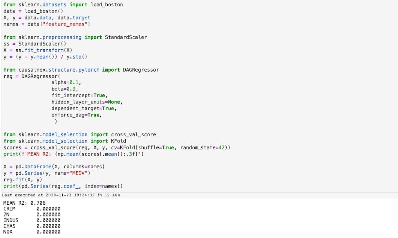
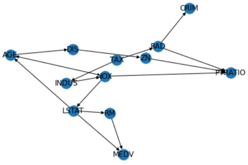
Provided this runs successfully we are then going to take the model that has been generated by the DAGRegressor algorithm to create a DAG using the Networkx library, which we will then visualise using some of the built in functions in Networkx.

import networkx as nx
dag = nx.DiGraph()

for col in list(names):
    s = reg.get_edges_to_node(col)
    for i in s.index:
        if s[i]>0:
            dag.add_edge(i, col, weight=s[i]);

s = reg.get_edges_to_node("MEDV")
for i in s.index:
    if s[i]>0:
        dag.add_edge(i, "MEDV", weight=s[i]);

from matplotlib import pyplot as plt

nx.draw(dag, arrows=True, with_labels=True)

Summary

We’ve now shown you how you can determine causation using Splunk with both the DLTK and SMLE, so it’s now over to you to see what use cases you can come up with using causal inference! Stay tuned for an approach using causal inference to determine root cause when analysing episodes in ITSI…

Happy Splunking!

For those interested in giving SMLE a try, SMLE Labs, our trial environment, is now seeking participants for the closed beta. Please visit the Splunk ML Environment (SMLE) Labs Beta page to sign up!