Efficiency Over Speed: Getting More Performance Out of Kafka Consumer

Splunk Infrastructure Monitoring is used to monitor modern infrastructure, consuming metrics from things like AWS or Docker or Kafka, and applying analytics in real time. Kafka is part of our core infrastructure. Being able to combine high throughput with persistence makes it ideal as the data pipeline underlying Splunk Infrastructure Monitoring's use case of processing high-volume, high-resolution time series. We do on the order of 50-60 billion messages per day on Kafka.

At the last Kafka meetup at LinkedIn in Mountain View, I presented some work we’ve done at Splunk Infrastructure Monitoring to get significant performance gains by writing our own consumer/client. This assume a significant baseline knowledge of how Kafka works. Note from the presentation are below along with the video embedded (start watching at 01:51:09). You can find the slides here (download for animations!).

The presentation was broken up into three parts:

1. Why we wrote a consumer
2. How modern hardware works
3. Three optimizations on the consumer
   
   

Why We Wrote a Consumer

We needed a non-blocking, single-threaded consumer with low overhead. The performance characteristics we were aiming for including consuming 100s or 1000s of messages per second, while dealing with GC. We are super sensitive to worst-case GC.

We don’t use the offset management or partition assignment functionality of Kafka, so our consumer is really meant to replace SimpleConsumer.

How Modern Hardware Works

A good way to think of modern processing systems is like distributed systems. On one end you have your number crunching cores and on the other your memory subsystems supplying the numbers and they’re all connected by a fast network.

In the past couple of decades, core speeds have gotten much faster then memory subsystems. So like all good distributed systems engineers, processor designers decided to add more caches. Solves everything. 🙂

A good rule of thumb on performance: the closer you get to a core, the faster–and smaller–a cache is:

• L1 – tiny, private to a core, segmented into data and instructions, fastest
• L2 – middling, private to a core, not segmented, less fast
• L3 – largest, shared by all cores, not segmented, slowest
   

It’s important to understand how data move around these memory systems to understand why we’ve gone down the road we have. Memory moves in fixed sized blocks called cache lines (on x64 this is usually 64B). If you’re trying to move even a single byte, the whole cache line will come along for the ride. So you better make it useful.

The memory subsystem makes three kinds of bets to optimize this process:

• Temporal locality: if you’ve used a piece of data, you’re very likely to use it again in the near future (like an LRU cache)
• Spatial locality: if you’ve used a piece of data, you’re very likely to use something close to it in memory (cache lines being 64B is an example itself)
• Prefetching: the processor tries very hard to figure out your memory access patterns and then tries to hide the inherent latency by pipelining cache fetches while you’re processing data—so any time you’re predictably accessing memory (like linearly walking an array), the processor will do this. 
  • Conversely, with unpredictable memory access access (like doing hashmap lookups), you get cache misses
     

The layout of data in memory can have a significant performance impact due to cache misses, because of the relatives speeds of the different stages of memory and the number of times you have to go to main memory. See 02:00:11 in the video for a demonstration and have a look at Jeff Dean‘s reference chart for latency, below. Memory latency is really what we’re fighting against and why we optimized our client implementation.

Optimizations on the Kafka Consumer

Our goal: have the consumer use as few resources as possible and leave more for the application.

We value efficiency more than raw speed (for the Consumer), because the real bottleneck there is in the network. We want to do more work with less resources, not more work faster. The resources we care about specifically are: cycles, cache usage / cache misses, memory.

Efficiency for the client translates into raw speed for the application.

All our efficiency gains came from applying constraints:

• No consumer group functionality needed
• A single topic that could be frozen as soon as the consumer was created (finite number of integer partitions)
• Partition reassignment is rare and only happens during startup or shutdown
• We are in complete control of the code that consumes the messages
   

Optimization 1: Use Cache Conscious Data Structures

Let’s explore this through an example: using arrays and open addressing hash maps.

We have a single topic, less than 1024 partitions, so all partitions implicitly belong to this topic. Partitions are simple integers, allowing us to use arrays instead of hash maps.

When we can’t use arrays, we try to use primitive specialized open addressing hash maps, which are much better than Java’s hash maps.

How we convert topic partitions to simple arrays:

• Assume you have an offset table
• Assume we have a single topic Foo, portioned 0-N, and it’s offsets
• Now our hash map is from an integer partition to an offset
• We know that N is the max number of partitions for that topic, so we convert this to a single sparse array with the index of the array equal to the partition
   

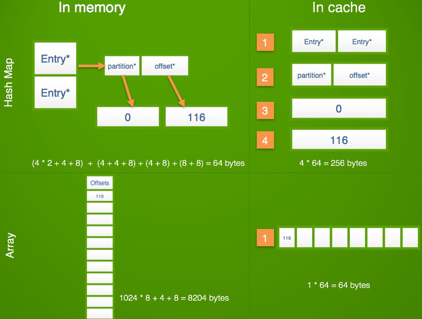
We’re avoiding Java hash maps because they’re implemented as an array of references to linked lists which themselves have references to keys and values. Let’s see what would happen with a simple get operation in a Java hash map for the above set up:

• Hash your key, which is a partition
• Land on a random offset, which is a cache miss because the location is completely unpredictable
• What you land on is a reference which needs to be followed, which is another cache miss (references lead to somewhere completely unpredictable)
• Check if the partition is equal to the one we were searching for, another cache miss
• Return the reference to the offset, not a cache miss
• But when you dereference that and get the offset, another cache miss
   

The Java hash map is a dependable cache miss generator.

Going back to our sparse array. Let’s say your trying to get the offset for the fourth partition: just load the fourth index, for a single cache miss

That’s four times less cache misses. But this is a tradeoff. The sparse array method takes way more memory, but way less cache. Something that uses 64B in memory can use 256B in cache (hash map), while something that uses 8KB in memory can use 64B in cache (sparse array). Cache is our rare resource, so the sparse array wins. This is not very intuitive.

All our data structures are built to be cache friendly. We try to prevent indirection and make everything boil down to walking an array, cause x86 processors are built for that.

The sparse array approach is not a good match for when you have multiple topics, so it’s not a very generalizable optimization. We think that using open addressing hash maps will be the better approach in the future.

Optimization 2: Create Buffers Once and Reuse

Remember we have a single topic with a finite number of partitions.

• As soon as you create the consumer, the topic and client string are immutable. They can be frozen. Anything that depends on that can be written once and used over and over.
• The metadata request buffer can be created just once
• Other requests can have their fixed parts written once
   

For a few examples of this reuse in actoion, see the video from 02:09:30 to 02:12:12.

Optimization 3: Zero Allocation Response Processing

Our messages have our own handwritten scheme and don’t need to be deserialized into Java objects. As soon as we’ve parsed a message, we pass it to the app. This is done without any copy or allocation at all. The benefits add up quickly when processing 100s of 1000s of messages per second.

The only problem with this is that it requires a fairly low-level interface. See an example at 02:14:41.

Results: 5000 Messages/Second at 218KB Mem and 2.63% CPU

Firstly, there are many Pareto-optimal choices here. Ours isn’t better, so much as it’s highly tuned for our workload. It can and will prove bad for other workloads.

Here are performance and resource consumption results from benchmarks we designed to test the client. Although we’re not fans of using benchmarks, in this case it was pretty much impossible to isolate Kafka performance vs everything else that’s running and doing work in the live app.

Benchmark set up:

• Single topic-partition
• Settings offetch_max_wait,fetch_min_bytes,max_bytes_per_partitionwere identical
• Only 5000 messages per second produced by a single producer
• Each message is 23 bytes
• Warm up, then profile for 5 mins 5000/sec * 5 mins = 1.5 million
   

All the consumer does is read a message, take out a few fields (longs), and write them somewhere in memory. We make sure it’s not optimized by the Java JIT. After a warm up, we profile for five minutes.

Looking at the allocation profile, the 0.9 Consumer does around 423MB for 1.5M messages (5000 per second), which is really good. A lot of those allocations are in message parsing and iterations. But we can make this go to complete zero. The benchmark took about 6.6% CPU, 6% being taken by the Consumer.

The Splunk Infrastructure Monitoring client allocates 218KB for 1.5M (5000 per second) messages, the entirety of which is from Java select call. We plan to use a Netty‘s version of the select call to completely get down to zero. This benchmark used about 2.63% CPU, with only 1.3% being taken by our client (our code using just 0.8% and the rest going to the Java select call).

We tried the same benchmark at 10,000 messages per second, with similar results.

Q&A

Do use multiple threads?
No, we have a single thread doing this. We divide work amongst threads, so one thread is responsible for an entire partition. So wherever we’re running this, we make sure there is no broker overlap.

Did you see any context switch cause core thrashing?
We bind our threads to a core using JNI, so we don’t see any context switches.

For memory improvements, can you specify which percentage comes from what optimization?
It’s very difficult to measure that. Especially for cache, you can’t measure which part of your code is taking how much cache. You can do some simplistic modeling, which is what we’ve done here. But this is based on math and not measurement.

Learn more about Splunk Infrastructure Monitoring and get an observability demo. 

Thanks,
Rajiv Kurian