ITSIのノイズ削減をさらにスマートに

今これをお読みになっている方の中にはさまざまな方がいらっしゃるでしょう。たとえば、グラフ分析でITSIのエピソードをさらにスマート化する方法について書いた前回のブログ記事を読んで機械学習の応用方法をもっと知りたいと思った方、強力なContent Pack for Monitoring and Alertingを使ってみたけれど依然として大量のアラートに悩まされている方、あるいは上司からAIOpsに関する調べ物を頼まれた方…。この記事にたどり着いた理由はそれぞれでしょうが、ここでは大量のアラートに潜む「未知の未知」を見つける方法をご紹介します。 

ITSIですでにイベント集約ポリシーを使用しており、十分に理解できている要因に基づいてアラートをグループ化できている場合でも、通常は見かけないような異常なアラートやアラートのグループを見つけ出すにはどうしたらいいか、お悩みの方もいらっしゃるのではないでしょうか。この記事ではその悩みにお応えしたいと思います。

「未知の未知」を見つけるにあたり、次の大きな2つの問いについて考えます。

1. アラートの量は特別に多いか？
2. アラートのタイプは異常なものか？

まずはそれぞれの問いを別々に検討してから、結果をまとめ、データの中に想定外の異常なイベントが大量に発生していないかを見極めます。

以降の手順ではいくつか大がかりなサーチが実行されるので、ご注意ください。

1.アラートの量は特別に多いか？

アラートの量が多いかどうかを判断する際には、以下の複数の観点から考える必要があります。

• このアラートの量はこの時間帯にしては異常に多いのか？
• このアラートの量はこのサービスにしては異常に多いのか？
• このアラートの量はサービスのこのコミュニティにしては異常に多いのか？

ここからは、Machine Learning ToolkitのProbability Density Functionを使って以上の3つの問いに答える方法について説明します。

以下のサーチは、任意のサービスの任意の時間帯、個々のサービス、そして個々のコミュニティラベルで想定されるアラートの量を基準とする、サービスの異常スコアを返します。

index=itsi_tracked_alerts 
| bin _time span=5m
| stats count as alerts by _time service_name
| join service_name type=outer [|inputlookup service_community_labels.csv | table src labeled_community | dedup src labeled_community | rename src as service_name]
| eval hour=strftime(_time,"%H")
| fit DensityFunction alerts by "hour" into df_itsi_tracked_alerts_volume as alert_volume_outlier
| fit DensityFunction alerts by "service_name" into df_itsi_tracked_alerts_service as service_alert_outlier
| fit DensityFunction alerts by "labeled_community" into df_itsi_tracked_alerts_community as community_alert_outlier
| eval anomaly_score=0
| foreach *_outlier [| eval anomaly_score=anomaly_score+<>]
| table _time alerts service_name anomaly_score *_outlier
| xyseries _time service_name anomaly_score 
| fillnull value=0

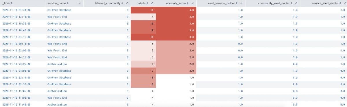
このサーチで以下のテーブルを得ることで、アラートの量が特に異常なサービスを特定できます。

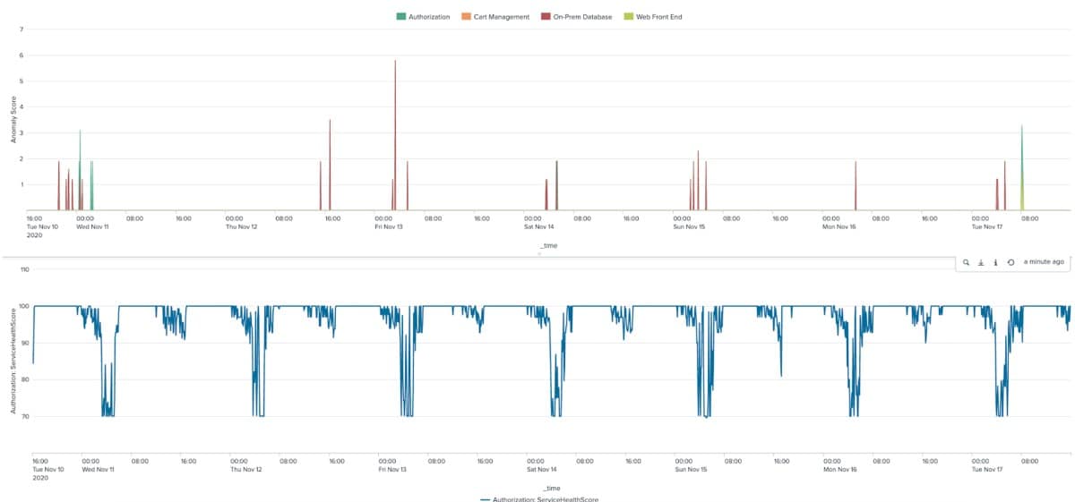
この結果を時間軸にプロットして異常スコアを確認することもできます。その場合は、サービス健全性スコアや、環境の健全性がわかるその他の指標と並べてみるとよいでしょう。

ただし、このサーチにはいくつか注意点があります。まず、データ内のサービスやコミュニティラベルの数が1,000を超えるような場合は、Splunkインスタンスへの負荷を抑えるため、Density Functionモデルのトレーニングはサービスやコミュニティごとに分けて行うことをおすすめします。

また、このサーチ結果からはアラートの量に関する情報しか得られず、アラートの中身についてはほとんど何もわからないことにも注意してください。次はアラートの内容に注目して、アラートタイプの組み合わせからサーチ結果を読み解けるかどうかについて考えます。

2.アラートの中身は異常か？

この検証は2段階で行います。

1. はじめに、各サービスのソースタイプの組み合わせを確認します。
2. 次に、Smart Ticket Insights App for Splunkを使って各サービスで発生しているアラートの記述内容を確認します。

2.1.ソースタイプの組み合わせ

ここでは、それぞれのサービスで5分ごとに記録されたアラートインデックスに現れる、各ソースタイプの数を見ます。以下のサーチで得られる統計はごく簡単なものですので、ご安心ください。

index=itsi_tracked_alerts 
| bin _time span=5m
| stats values(orig_sourcetype) as sourcetypes by _time service_name
| eval sourcetypes=mvjoin(mvsort(sourcetypes),"|")
| stats count by sourcetypes service_name
| eventstats sum(count) as total by service_name

サーチ結果は以下のようになります。

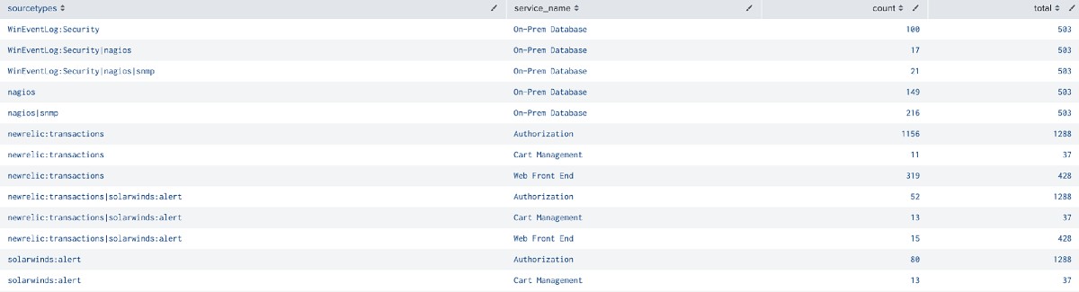
合計数に対するアラート数の割合を見ると、各サービスでそのソースタイプの組み合わせが発生する頻度が見えてきますが、ひとまずこの結果をルックアップ「expected_itsi_alert_sourcetypes.csv」として保存します。このファイルは後でまた使用します。

2.2 アラートの説明の分析

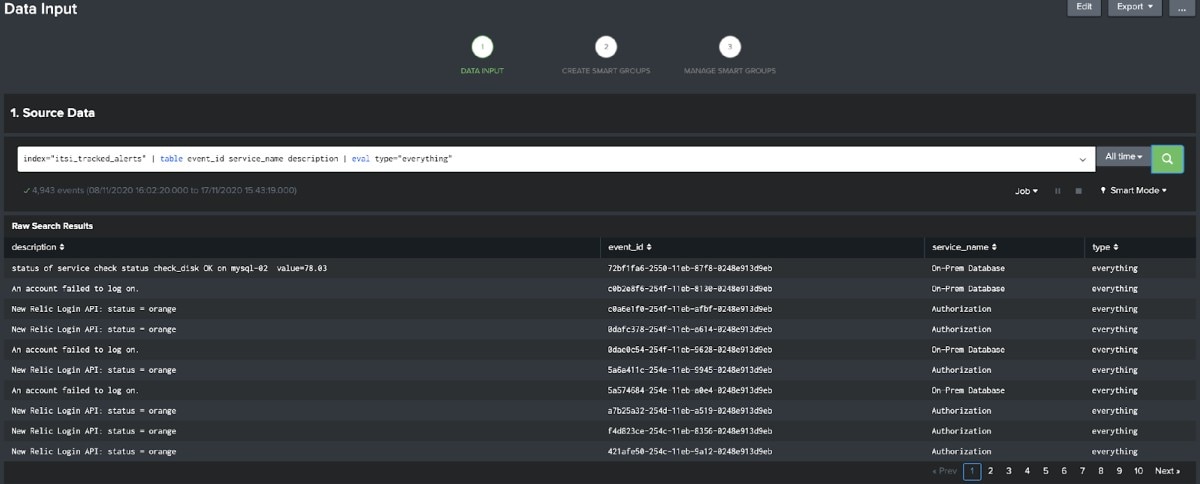
次に、Smart Ticket Insights App for Splunkを使って、データに含まれるアラートの通常の記述内容を定めます。このAppについて詳しくはこちらをご覧ください。まずは簡単なサーチを実行して、相関サーチインデックスからアラートの説明、ID、サービス名を取得します。

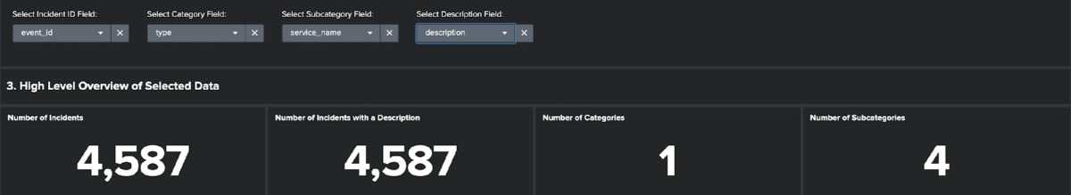
以下の画像のように目的のフィールドを各ドロップダウンで選択すると、そのデータのレポートが得られます。パネルにデータが表示されたら、ドロップダウンからしきい値を1つ選択し、[Identify Frequently Occurring Types of Tickets]ボタンをクリックします。

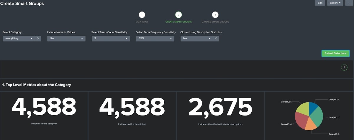
次のダッシュボードでは、絞り込んだグループに応じて選択内容を調整することをおすすめします。以下の画像では基本的にデフォルトの選択をそのまま使用し、[Cluster Using Description Statistics]の選択肢のみオフにしています。グループを確認してアラートのグループ化が妥当だと思えば、モデルを保存し、[Manage Smart Groups]ダッシュボードに移動します。

[everything]カテゴリを選択すると先ほどと同様のレポートが再度表示されますが、グループを選択すると[open in search]ボタンが表示されます。このボタンをクリックすると、以下のようなサーチが新しいウィンドウで開きます。ただし、以下のサーチは生成されたものそのままではなく、適宜編集してあります。具体的には、サーチ全体に_timeフィールドを追加し、最後の数行を統計計算用のコマンドに変更しています。

index="itsi_tracked_alerts" | table _time event_id service_name orig_sourcetype description | eval type="everything"
| table _time "event_id" "type" "service_name" "description"
| rename "event_id" as documentkey "type" as category "service_name" as subcategory "description" as description
| eval category=if(category="","No Category",trim(category)), subcategory=if(subcategory="","No Subcategory",trim(subcategory))
| where NOT ( subcategory="$result.exclude$")
| eval category=replace(replace(category,"[^A-Za-z0-9| ]","")," ","_")
| search category="everything"
| eval descriptionmv=description, description_fragment=description
| makemv delim=" " descriptionmv
| eval PC_description_length=len(description), PC_words=mvcount(descriptionmv)
| fields - descriptionmv
| rex field=description_fragment mode=sed "s/([\r\n]+)/|/g"
| makemv delim="|" description_fragment
| eval PC_lines=mvcount(description_fragment)
| mvexpand description_fragment
| eval description_fragment_len=len(description_fragment)
| makemv delim=" " description_fragment
| eval words_line=mvcount(description_fragment)
| fields - descriptionmv
| stats max(PC_description_length) as PC_description_length max(PC_words) as PC_words max(PC_lines) as PC_lines avg(description_fragment_len) as PC_avg_line_length avg(words_line) as PC_avg_words_per_line by _time documentkey category subcategory description
| apply tfidf_ticket_categorisation_everything_1605112121
| apply pca_ticket_categorisation_everything_1605112121
| apply gmeans_ticket_categorisation_everything_1605112121
| rename cluster as gmeans_cluster
| join type=outer category gmeans_cluster [| inputlookup ticket_cluster_map.csv]
| table _time documentkey category subcategory description filter_cluster
| eval filter_cluster=if(len(filter_cluster)>0,filter_cluster,"No cluster")
| bin _time span=5m 
| stats values(filter_cluster) as groups by _time subcategory
| eval groups=mvjoin(mvsort(groups),"|")
| stats count by groups subcategory
| eventstats sum(count) as total by subcategory

このサーチは、上で示したソースタイプのテーブルと非常によく似たテーブルを返します。

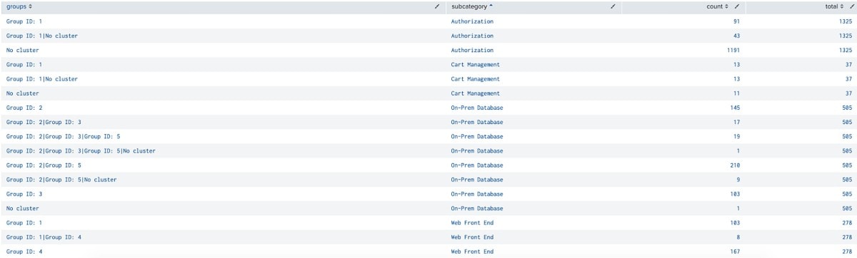
これで、相関サーチを実行した各サービスで想定されるアラートの説明のデータが得られました。この結果をルックアップ「expected_itsi_alert_groups.csv」として保存します。

3.結果をまとめる

以下の長々としたサーチには少々面食らうかもしれませんが、大部分はSmart Ticket Insights App for Splunkで自動生成されたもので、いくつかの行に手を入れ、目的の結果を得るための統計計算コマンドを最後に追加しただけです。具体的には、サーチ全体にorig_sourcetypeフィールドを追加しました(太字でハイライトした箇所)。それから、目的の統計を計算するために、グループが割り当てられていないアラートを返すevalステートメントの後ろの部分をすべて書き換えました。また、Density Functionモデルを適用し、この記事のセクション2で生成したルックアップを用いた結果のエンリッチ化も行っています。

index="itsi_tracked_alerts" | table _time event_id service_name orig_sourcetype description | eval type="everything"
| table _time "event_id" "type" "service_name" "description" orig_sourcetype
| rename "event_id" as documentkey "type" as category "service_name" as subcategory "description" as description
| eval category=if(category="","No Category",trim(category)), subcategory=if(subcategory="","No Subcategory",trim(subcategory))
| eval category=replace(replace(category,"[^A-Za-z0-9| ]","")," ","_")
| search category="everything"
| eval descriptionmv=description, description_fragment=description
| makemv delim=" " descriptionmv
| eval PC_description_length=len(description), PC_words=mvcount(descriptionmv)
| fields - descriptionmv
| rex field=description_fragment mode=sed "s/([\r\n]+)/|/g"
| makemv delim="|" description_fragment
| eval PC_lines=mvcount(description_fragment)
| mvexpand description_fragment
| eval description_fragment_len=len(description_fragment)
| makemv delim=" " description_fragment
| eval words_line=mvcount(description_fragment)
| fields - descriptionmv
| stats max(PC_description_length) as PC_description_length max(PC_words) as PC_words max(PC_lines) as PC_lines avg(description_fragment_len) as PC_avg_line_length avg(words_line) as PC_avg_words_per_line by _time documentkey category subcategory description orig_sourcetype
| apply tfidf_ticket_categorisation_everything_1605112121
| apply pca_ticket_categorisation_everything_1605112121
| apply gmeans_ticket_categorisation_everything_1605112121
| rename cluster as gmeans_cluster
| join type=outer category gmeans_cluster [| inputlookup ticket_cluster_map.csv]
| table _time documentkey category subcategory description filter_cluster orig_sourcetype
| eval filter_cluster=if(len(filter_cluster)>0,filter_cluster,"No cluster")
| bin _time span=5m 
| stats count as alerts values(filter_cluster) as groups values(orig_sourcetype) as sourcetypes by _time subcategory
| eval sourcetypes=mvjoin(mvsort(sourcetypes),"|"), groups=mvjoin(mvsort(groups),"|"), hour=strftime(_time,"%H")
| join subcategory type=outer [|inputlookup service_community_labels.csv | table src labeled_community | dedup src labeled_community | rename src as subcategory]
| rename subcategory as service_name
| apply df_itsi_tracked_alerts_volume 
| apply df_itsi_tracked_alerts_service 
| apply df_itsi_tracked_alerts_community 
| eval anomaly_score=0
| foreach *_outlier [| eval anomaly_score=anomaly_score+<>]
| lookup expected_itsi_alert_sourcetypes.csv sourcetypes as sourcetypes service_name as service_name OUTPUTNEW count total
| lookup expected_itsi_alert_groups.csv groups as groups subcategory as service_name OUTPUTNEW count as group_count total as group_total
| eval sourcetype_likelihood=1-(count/total), group_likelihood=1-(group_count/group_total)
| eval anomaly_score=anomaly_score*(sourcetype_likelihood+group_likelihood)
| table _time service_name alerts anomaly_score *_outlier *_likelihood

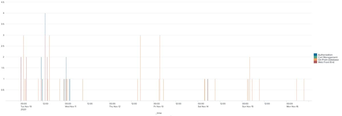
このサーチは、異常スコアを含む結果を返します。異常スコアは、「外れ値の合計個数」と「データにおけるそのソースタイプとアラートグループの組み合わせの発生確率」の積です。

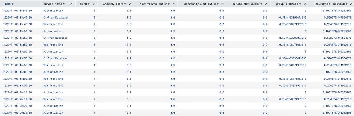
このテーブル自体からはそれほど得るものはありませんが、異常スコアといずれかのサービス健全性スコアを並べてみると、はっきりとした相関が浮かび上がってきます。どうやら、サービス健全性スコアが低下した時間の前後で異常なパターンが発生しているようです。この情報をもとにアラートをたどって環境内で起きていることを具体的に調べていけば、根本原因を突き止められるかもしれません。

まとめ

このブログ記事では、統計分析を使ってイベントの発生数が異常かどうかを判断する方法と、同様の手法を、説明文とソースタイプの組み合わせが異常かどうか、といった非数値データへ適用する方法について説明しました。このように複数の手法を組み合わせることで、サービスのパフォーマンス低下に関係している可能性のあるイベントの大量発生を見つけ出すことができ、これは本当に重要なアラートを突き止めることに役立ちます。

ぜひ、ここでご紹介した内容をもとにイベントデータに対して教師なし機械学習を実行して、相関サーチ結果の中に隠れたパターンがないかチェックしてみてください。

Splunkのメリットをどうぞお試しください。

このブログはこちらの英語ブログの翻訳、沼本 尚明によるレビューです。