How To Choose a Vector Database Architecture

The vector database you choose will shape your RAG system's cost, latency and recall more than almost any other component. It is also the decision teams tend to make first and revisit last, usually after the corpus has grown past the point where the original choice still fits.

This article is about the structural half of that decision — the part you commit to before a single query runs. How vectors get indexed, what that index costs in memory, how far compression can take you, and which databases are built for which shape of problem. Get these right and the system scales; get them wrong and no amount of query-time tuning compensates.

The query-time half — filtering, hybrid search, model integration and what to monitor once traffic arrives — is covered separately in Operationalizing Your Vector Database for Production RAG.

What a vector database does

A vector database solves one specific problem: finding the nearest neighbors to a query vector among millions or billions of stored vectors.

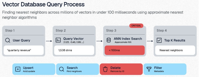
Traditional databases are built for exact matches and range filters. A B-tree index works well for user IDs or timestamps because those operations map cleanly onto comparison operators. Embedding-based retrieval has a different access pattern entirely. When a user asks about quarterly revenue, your system converts that question into a 1,536-dimensional vector and searches for similar vectors across the whole corpus. Computing exact distances between the query and every stored vector scales linearly with corpus size — at one million vectors, that is more than a billion floating-point operations per query.

Vector databases get around this with approximate nearest neighbor (ANN) indexes. These trade exact recall for speed, returning vectors that are close enough to the true nearest neighbors for retrieval to work in practice. With a well-configured index, you can search millions of vectors in under 100 milliseconds.

Choosing the right vector database

Choosing a vector database comes down to three questions answered in order.

1. How many vectors will you have, once you multiply documents by chunks?
2. Do you have a team that can run database infrastructure?
3. What is the one requirement you cannot compromise on — filtering, scale, on-premises hosting, or simply that it works reliably without much attention?

Answer those and the field narrows to two or three candidates, at which point index structure, quantization strategy, and filtering behavior tell you which one fits, and this article walks you through these choices.

Finally, get the sizing math right before you commit, because the difference between an index that fits in memory and one that does not is the difference between a system you tune and a system you rebuild.

Four core vector database operations

Four core operations of vector operations do most of the work. They look simple, but their performance depends almost entirely on how vectors are indexed.

Distance metrics

Vector similarity depends on a distance metric to quantify how close two vectors are. The choice affects both retrieval quality and computational cost.

• Cosine similarity measures the angle between vectors and ignores magnitude. This suits embeddings where direction matters more than scale, which is why most text embedding models optimize for it.
• Euclidean distance measures straight-line distance in vector space, accounting for both direction and magnitude. Use it when vector length carries meaning, as it does in some image embeddings.
• Dot product sums the element-wise multiplications, combining angle and magnitude. Some databases optimize dot product operations heavily, making them faster than cosine similarity in practice.

Modern vector databases support all three. For text, cosine similarity is the usual choice, because embedding models are designed to place similar meanings in the same direction even when their lengths differ.

Index structures

Vector databases differ primarily in how they index vectors for similarity search. This single architectural choice determines recall, latency, memory usage and update behavior. Four approaches dominate production systems: flat indexes, HNSW, IVF, and DiskANN.

Different databases commit to different index families, and that commitment is often the real constraint on what you can tune later.

Flat indexes

Flat indexes store vectors with no additional structure. For each query, the system computes the distance between the query vector and every stored vector, then returns the top-k closest results. This guarantees 100% recall, with performance that scales linearly — searching 100,000 vectors takes roughly ten times longer than searching 10,000.

Because there is no graph to traverse, flat indexes work well for small collections, typically under 100,000 vectors. They are common in prototypes and small retrieval augmented generation (RAG) systems. As the corpus grows, exhaustive distance computation stops being practical and approximate methods become necessary.

HNSW (Hierarchical Navigable Small World)

HNSW organizes vectors into a multi-layer graph built for fast approximate search. Queries traverse from coarse to fine layers, narrowing the search space quickly. The design achieves high recall at low latency and is the default in most production systems running millions of vectors.

The tradeoff is memory. HNSW's speed comes from keeping the entire graph structure in RAM, and the graph connections multiply memory requirements well beyond the cost of storing the vectors themselves. Systems with millions of vectors need substantial memory; billion-vector deployments become expensive fast. Parameters such as M and efConstruction control the balance between recall, build time and memory overhead.

IVF (Inverted File Index)

IVF partitions the vector space into clusters and assigns each vector to its nearest centroid. At query time the system searches only the most relevant clusters. This keeps centroids in RAM while storing full vectors on disk, which supports far larger corpora than HNSW on the same hardware — often tens or hundreds of millions of vectors. Retrieval quality depends on clustering quality and the nprobe setting, which trades recall against latency.

DiskANN

Built on the Vamana graph algorithm, DiskANN extends graph-based search by keeping a compressed index in memory and the full vectors on SSD, loading them only for final distance calculations. Shifting memory pressure from RAM to disk makes billion-scale vector search feasible on commodity hardware. You give up some latency in exchange for large memory savings, and you get more stable performance under frequent updates than a fully in-memory graph index provides.

Index choice: How to size your index before choosing

Most index decisions come down to whether the index fits in memory. You can work that out in four steps:

1. Multiply document count by average chunks per document.
2. Multiply chunk count by embedding dimension.
3. Multiply by 4 bytes per float32 value.
4. Add index overhead — 2-3x for HNSW, 0.2-0.5x for IVF.

Take a corpus of 100,000 documents averaging five chunks each. That yields 500,000 vectors.

• At 1,536 dimensions, each vector needs 6KB, so raw vectors come to 3GB.
• HNSW adds 6-9GB for the graph structure, totaling 9-12GB.
• IVF adds only 0.6-1.5GB, totaling 3.6-4.5GB.

If your calculated memory exceeds available RAM, IVF or DiskANN becomes necessary. If you have the memory to spare, HNSW gives you better recall and latency for it.

Modern models (like OpenAI's text-embedding-3 or latest open-source models) support Matryoshka Embeddings. This allows you to truncate a 1,536-dimensional vector down to 256 or 512 dimensions with minimal loss in recall. This is the most effective way to reduce memory costs before even applying quantization.

Quantization techniques

Index choice determines how you search vectors. Quantization determines how many you can store by reducing memory usage by lowering vector precision. At scale, quantization is now a requirement, not only an optimization. Let’s look at three common techniques.

Binary quantization

Binary quantization converts each vector dimension into a single bit based on its sign. Similarity comparisons then run on binary codes using fast bitwise operations. Binary representations preserve coarse directional similarity but lose fine-grained distance information, which limits ranking quality. It works best in large-scale retrieval systems where throughput and memory efficiency matter more than exact ordering, and it is often paired with graph-based indexes to recover accuracy.

Product quantization

Product quantization compresses vectors by splitting them into subvectors and quantizing each subspace independently. The system stores compact codes referencing precomputed centroids rather than full precision values, and approximates distances at search time using lookup tables. This delivers substantial memory savings while retaining useful distance information, which is why it shows up in very large document and image collections.

Scalar quantization

Scalar quantization converts floating-point values into lower-precision integers such as int8 or int4. It lowers memory usage significantly while preserving the structure of the vector space more faithfully than binary methods. Because relative distances survive, many systems adopt it as a default compression strategy when moderate savings are enough. It fits interactive workloads that need to balance latency, memory and retrieval quality.

Choosing managed services vs. self-hosting

Before comparing specific databases, settle the deployment question. It shapes everything downstream, from operational overhead, cost structure, to control, and it narrows the field considerably. Neither option dominates.

• Managed services handle infrastructure, scaling, backups and monitoring, which lets teams deploy production systems without specialized database expertise. Usage-based pricing keeps costs predictable for stable workloads. Multi-region deployments rely on provider-managed replication and failover, removing a large chunk of operational complexity.
• Self-hosting gives you full control over configuration, updates, and data residency, which matters in regulated environments and anywhere data has to stay on-premise. Cost shifts from variable to fixed, and at large scale self-hosting often ends up cheaper than per-query pricing. It also enables deeper customization, from kernel tuning to proprietary integrations.

Common production vector databases

With a deployment model decided, you can evaluate specific databases on their strengths and operational characteristics.

• Pinecone. Fully managed: you create an index, set the dimension and distance metric, and Pinecone handles infrastructure and scaling. The serverless tier scales with usage; the pod-based tier trades that for dedicated resources and more predictable performance.
• Weaviate. Stores data as connected objects, so similarity search runs alongside relationship traversal. Hybrid search and generative search are both native, which makes it the strongest fit for knowledge-graph and schema-driven retrieval.
• Qdrant. Builds filtering directly into the HNSW index, so performance holds up under complex Boolean conditions. Quantization can be applied selectively, letting you run compressed search with full-precision reranking.
• Milvus. Separates compute and storage and runs on Kubernetes, so each layer scales independently to billions of vectors. Supports HNSW, IVF and DiskANN, with GPU acceleration for both search and index construction.
• pgvector. Adds a vector type and similarity indexes to PostgreSQL, so vectors sit beside your relational data and inherit its joins, transactions, backups and access control. One database instead of two matters more than benchmark numbers, right up until you hit the scale that demands a specialized system.
• MongoDB Atlas Vector Search. Stores embeddings next to your operational data, so a single Atlas cluster serves as both primary database and vector store. Supports approximate search via HNSW and exact nearest neighbor and combines vector search with standard MongoDB filters and aggregation.

Choosing by constraint

In practice, vector database selection is driven less by raw retrieval quality than by operational constraints. Deployment model, filtering requirements and existing infrastructure usually narrow the field before performance differences matter.

The enterprise evaluation checklist

Beyond technical architecture, most production deployments prioritize compliance and access control. Evaluate these requirements early. A database that meets your technical needs but lacks a required certification creates deployment delays that no amount of benchmarking will fix. Choosing purely on compliance without validating technical fit produces the opposite problem.

Agent observability with Splunk

Choosing your vector database settles the structure. What it does not settle is behavior under real traffic — how metadata filters interact with the index you just picked, whether keyword matches survive a purely semantic search, and what degradation looks like six months in when the corpus has doubled. Those are query-time problems — and that’s where most RAG systems actually lose ground.

Understanding AI agents at work is key to trusting AI systems. Learn about Splunk Agent Observability and get hands-on with the Splunk Observability Cloud Free Edition today

FAQs about vector database selection