How to Architect an Enterprise Retrieval-Augmented Generation (RAG) System

Your RAG demo worked. In production, it confidently cites a paper that never made the claim. Barnett et al. cataloged seven common RAG failure points, and newer work has widened that picture.

7 common failure points of RAG systems

RAG pipelines break down, and there are seven common points of failure, from retrieval gaps to generation slip-ups.

• Missing content (FP1): Documents can't answer the question; the system answers anyway.
• Missed the top-ranked documents (FP2): The answer is in the corpus but never ranks inside the top K.
• Not in context (FP3): The chunk was retrieved, then dropped during context consolidation.
• Not extracted (FP4): The answer is in context, but noise or conflict hides it.
• Wrong format (FP5): You asked for a table; the model ignored it.
• Incorrect specificity (FP6): The answer is too general or too specific.
• Incomplete (FP7): Accurate but omits information from context.

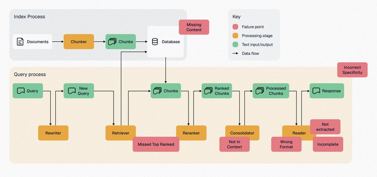
Leung et al. extended this taxonomy at EACL 2026 to 16 error types across chunking, retrieval, reranking, and generation after finding a 27% error rate on DragonBall-EN. They found fabricated content “relatively rare” compared with retrieval and chunking errors.

Read that ranking as a triage order. If your first instinct when an answer is wrong is to rewrite the system prompt, you are starting at the stage where errors are least likely to originate.

How to build an enterprise RAG system: The complete stack

A production-grade RAG stack layers authentication, guardrails, retrieval, generation, and observability into a single end-to-end pipeline.

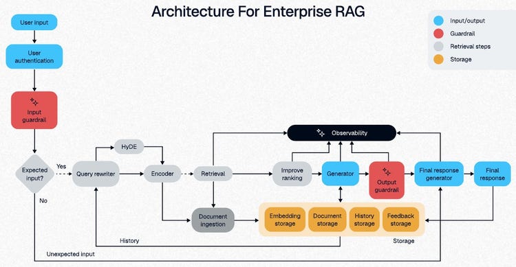
User authentication

Authenticate before retrieval for access control, compliance, and auditing. Identity becomes the metadata filter scoping retrieval per tenant.

Input guardrail

Block harmful or private inputs: personally identifiable information, injection substrings, executable code, off-limit topics, oversized prompts, and toxicity. PoisonedRAG (USENIX Security 2025) hit a 97% black-box attack success rate against PaLM 2 on Natural Questions (NQ) with five malicious texts in a 2.68 million-text database.

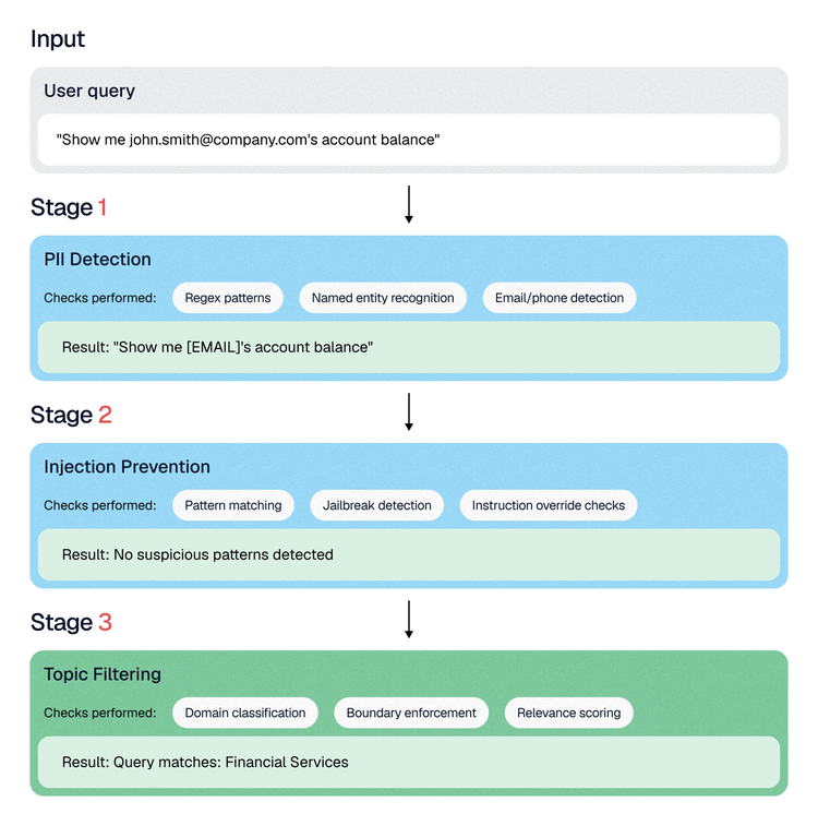
Meta's suite is Llama Guard 4, a 12 billion-parameter multimodal classifier with the S1–S14 hazard taxonomy, plus Prompt Guard 2 (86 million and 22 million parameters) for injection and jailbreak detection. In an ICLR 2026 workshop benchmark of 79,331 samples, Llama Guard (12 billion parameters) scored 0.47 F1 against 0.76 for Qwen Guard (4 billion parameters).

Query rewriter

Rewrite vague queries after the guardrail clears.

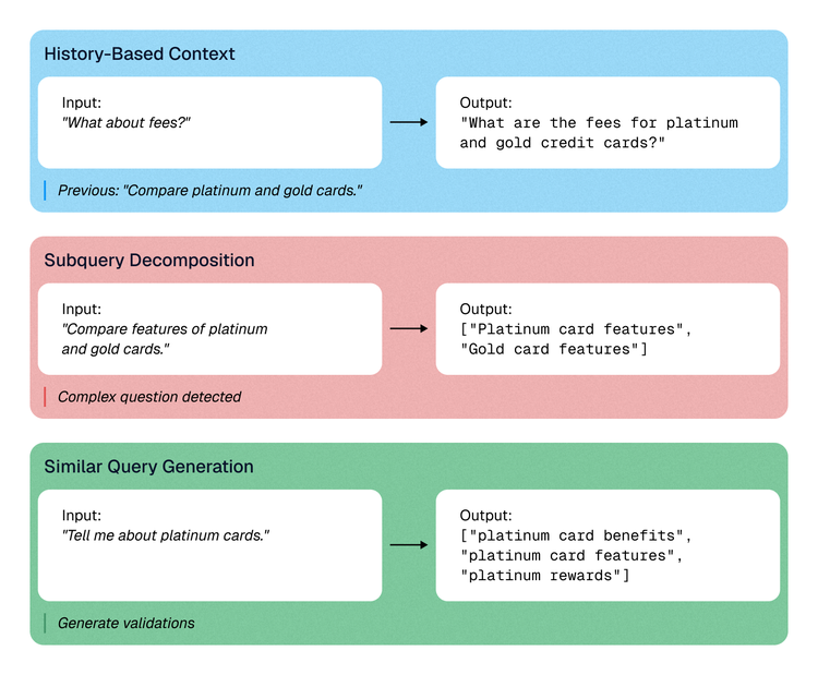
Rewrite based on history. “Compare features of both.” becomes “Compare features of platinum and gold credit cards.”

Create subqueries. Split it by card type. LlamaIndex implements this as the SubQuestionQueryEngine. At ACL 2025 SRW, decomposition with reranking lifted mean reciprocal rank at 10 (MRR@10) by 36.7% and answer F1 by 11.6% on MultiHop-RAG and HotpotQA.

Create similar queries. “I want to know about platinum credit cards” becomes “platinum credit card benefits.” An EMNLP Industry Track study found a union of four rewriting methods raised enterprise hit rate at 10 (HIT@10) from 39.22 to 51.7, and a confidence-gated router captured +4.3 points while rewriting fewer than 40% of queries at about 40% of full expansion cost.

That router result is the one to copy. Rewriting every query buys a little accuracy at full cost and full latency; gating on confidence buys most of the accuracy on the minority of queries that need it, which is also what keeps the rewrite stage inside its latency budget.

Encoder

Encoder choice is critical. The Massive Text Embedding Benchmark (MTEB) comprises MTEB(eng, v2) and the multilingual benchmark, covering 500 tasks across 250+ languages, where instruction-tuned models outperform the rest.

OpenAI's text-embedding-3-large supports Matryoshka truncation from 3072 dimensions to 256 while still beating unshortened ada-002 on MTEB, at $0.13 per million tokens. Open-source Qwen3-Embedding-8B (Apache 2.0) scored 70.58 on MTEB multilingual at release.

Beyond leaderboard scores:

• Storage and latency. Both scale with dimension, so truncate to 256–768 and store embeddings separately so migrations never force re-encoding.
• Language support. Multilingual corpora need a multilingual encoder or upfront translation.
• Privacy. Finance and healthcare rules may prohibit external application programming interfaces (APIs).

MTEB won't predict domain performance. Score mean reciprocal rank and normalized discounted cumulative gain (nDCG) on an annotated gold set, use a cross-encoder as a judge, or cluster with hierarchical density-based spatial clustering of applications with noise (HDBSCAN).

Document ingestion and chunking

IBM's Docling handles PDF, Office documents, HTML, and images with layout analysis and TableFormer table recognition, measured by tree-edit-distance-based similarity (TEDS), which reaches 96.75% TEDS on PubTabNet.

A NAACL study found fixed-size chunking beat semantic chunking on three of five datasets; a 36-strategy benchmark across six domains and five embedding models put paragraph grouping at a mean nDCG@5 of about 0.46 versus 0.24 for fixed character splits. Anthropic's contextual retrieval cut top-20 retrieval failures by 35% alone, 49% with contextual BM25, and 67% with reranking added.

Those two findings are not in conflict, though they are often quoted as if they were. Semantic splitting is not reliably better than fixed-size splitting; paragraph grouping — respecting the document's own structure — is. Boundary quality is what moves retrieval, not the sophistication of the algorithm that finds the boundary.

Indexer and data storage

The indexer maps chunks to locations and handles creation, updates, and deletion. Store embeddings in the vector database, documents in object storage, and chat history in a relational or NoSQL table to avoid recomputation during reindexing.

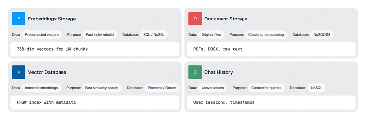
Vector database

Recall vs. latency

Hierarchical Navigable Small World (HNSW) is the default graph index in Milvus, pgvector, and Weaviate. Milvus ships M=30 and efConstruction=360; higher M buys recall with memory, while higher efConstruction buys quality with build time.

In-memory vs. on-disk

DiskANN searched a billion vectors at over 5,000 queries per second with under 3ms latency on 64GB RAM plus a solid-state drive (SSD) in its original benchmark. Quantization is another lever: BBQ offers about 32x compression for dense vectors of 384+ dimensions.

Hybrid search

Combine a dense index, sparse inverted index, and fusion step; Weaviate defaults to relativeScoreFusion with alpha 0.75.

Filtering

Pre-filtering can miss results; post-filtering breaks on rare attributes. ACORN-style predicate-aware traversal mitigates both and is Weaviate's default HNSW filter strategy in v1.34.

Techniques for improving retrieval

NoLiMa showed 11 of 13 models fell to half or less of their short-context baseline at 32,000 tokens, with GPT-4o falling from 99.3% to 69.7%. EKRAG found enterprise accuracy improves from one to five retrieved chunks, then plateaus or reverses from five to 10.

HyDE: Embedding a hypothetical answer helps sparse retrieval most: at SemEval it improved BM25 by 26.7% but dense retrieval by only 4.0%.

Query routing: Route each query to the relevant index before searching.

Reranker: Rerankers matter most when the first stage is weak: RankZephyr gained 45–55% over top-100 BM25 candidates but only 7–20% over SPLADE++. On 1,200 U.S. Securities and Exchange Commission (SEC) filings, cross-encoder reranking lifted MRR@5 from 0.160 to 0.750 at 2.02 seconds average latency, while small-to-big retrieval won 65% of comparisons for 0.2 seconds of added latency.

A caveat on that 2.02 seconds, because it gets quoted out of context: it is the average end-to-end latency reported for that study's pipeline over long SEC filings, not the incremental cost of the reranking stage. Budget a cross-encoder at roughly +200–400ms on ordinary chunk sizes, a late-interaction model such as ColBERT at +150–300ms, and an LLM listwise reranker at +4–6 seconds. Then measure on your own corpus, because document length drives all three.

Maximal Marginal Relevance: DF-RAG reports 4–10% F1 gains from MMR-style selection on reasoning-intensive question answering (QA), and diverse documents improved correctness by 17–47% where duplicates did not.

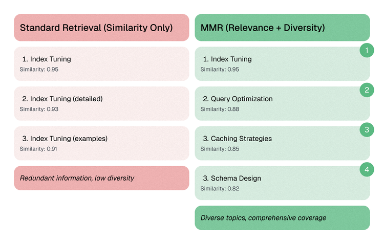
Maximal Marginal Relevance trades a little per-chunk similarity for coverage, so near-duplicates don't consume the context window.

Autocut: Truncate result lists at score discontinuities, as Weaviate's autocut does.

Recursive and sentence window retrieval: Embed small chunks and return the parent chunk or text window via LlamaIndex's RecursiveRetriever and SentenceWindowNodeParser. DER-RAG shows isolated sentences lose their referents.

Generator

Hugging Face has archived Text Generation Inference and points users to vLLM, whose automatic prefix caching suits long-prefix RAG prompts, and SGLang, whose prefill-decode disaggregation reports 2–5x throughput gains at high concurrency.

Measure time to first token (TTFT) and time per output token (TPOT) as vLLM defines them; the Anyscale LLMPerf leaderboard is archived, while MLPerf Inference is the active benchmark and requires 99th-percentile TTFT under six seconds and TPOT under 175ms for Llama 3.1 405B server. Pricing splits input, cached input, and output, with batch APIs at 50% off, so weigh Claude Sonnet 5 at $2/$10 per million tokens against GPU cost and utilization.

Latency budgets and parallelization

TTFT and TPOT describe the generator. They say nothing about the seven stages in front of it, and in most enterprise pipelines those stages own more of the wall clock than generation does. Latency is a design constraint you set when the system is first assembled, not an optimization you apply once it is slow.

Production systems define an explicit budget for each stage — query processing, retrieval, reranking, generation, validation — and the budget decides three things about every operation: whether it must complete before the response can proceed, whether it can run in parallel, and whether it can run after the response has already been delivered.

Much of the retrieval layer parallelizes cleanly. Queries can fan out to multiple indexes at once — technical documentation, product content, structured data stores — so the cost is the slowest index, not the sum of all of them. Reranking and filtering can start on partial results as soon as the first index returns, rather than waiting for every call to land.

Other operations are sequential by necessity. Query rewriting has to finish before retrieval begins. Generation cannot start until enough context is available. Blocking output validation has to complete before anything is returned. But logging, evaluation and feedback collection can all run after the response has been delivered, and moving them off the critical path is usually the largest single latency win available.

Streaming reduces perceived latency further by returning tokens as generation begins, while non-blocking checks continue in parallel — provided every blocking guardrail has executed before streaming starts.

An illustrative budget for a two-second target, to be replaced with measurements from your own corpus:

Without parallel execution and explicit budgets, well-designed retrieval and generation components still miss production requirements — because nobody ever decided what the pipeline was allowed to spend.

Output guardrail and user feedback

The output guardrail catches hallucinations, competitor mentions, and brand damage. NeMo Guardrails supports input, dialog, retrieval, execution, and output rails in one configuration.

Collect thumbs, ratings, and free text, then diagnose whether failures came from retrieval, generation, or data. Fixing data pays most; add each fixed query to the test suite.

Observability

Splunk Agent Observability splits RAG trace metrics into retrieval quality and generation quality, scored separately on the same trace.

• Chunk Relevance is binary and per chunk: each retrieved chunk comes back Relevant or Not Relevant. If nothing is Relevant for a query, retrieval failed for that query, and no amount of prompt work will fix the answer.
• Context Relevance asks the same question of the retrieved context as a whole — does it contain enough to answer? Start here, then drill into Chunk Relevance to find which chunks let you down.
• Context Precision weights the relevant share of the context by rank position; Precision @ K does the same at a fixed cut-off. Together they answer how much of what you retrieved was worth retrieving.
• Context Adherence catches closed-domain hallucinations — did the response stay inside the context it was given?
• Completeness measures how thoroughly the response covered the relevant context. If Context Adherence is precision, Completeness is recall.

The scoring lineage traces back to the Chainpoll paper, originally from Galileo. Read that as provenance rather than mechanism: the Luna evaluation models running in production today are fine-tuned Llama models that score with log-prob classification, not a frontier model polled several times.

Those evaluators run on Luna evaluation models at under 200ms and at up to 96% below the cost of using a frontier large language model (LLM) as a judge. Traces arrive through LangChain callbacks, LlamaIndex, and OpenTelemetry and OpenInference.

If you are instrumenting directly rather than through a framework callback, the span type is what tells the platform which evaluators apply to which stage:

Then turn on the evaluators you want running against that agent stream. Because evaluation is off the critical path, this is where the retrieval scores get computed without spending the user's latency budget:

One thing to watch: enable_evaluators replaces the whole set each time it runs. List every evaluator you want active, not just the one you are adding, or you will silently switch the others off.

Caching

OpenAI's prompt caching automatically cuts input cost up to 90% above a 1,024-token minimum; GPTCache handles semantic caching but its maintainers “no longer add support for new API or models.”

Advanced RAG

Agentic RAG

Agentic RAG decides when to search, decompose tasks, and call tools. In an ACL Industry Track study, agentic settings used 3.3x more input tokens, 1.9x more output tokens, and 1.5x more time than enhanced RAG. Standard RAG takes two to three seconds, compared with eight to 15 seconds for agentic RAG with three to five tool calls. Reserve it for multi-hop queries.

Notice that those numbers put agentic RAG an order of magnitude outside the latency budget above. That is the real decision: not whether agentic retrieval answers better, but whether the query class justifies a different budget entirely.

Graph RAG

Microsoft's GraphRAG global search won 72–83% of “comprehensiveness” comparisons against naive RAG on the podcast dataset, at 331,375 tokens per query versus 879 for vanilla RAG. LazyGraphRAG indexes at 0.1% of that cost and queries at more than 700× lower cost.

Multimodal RAG

On UniDoc-Bench (70,000 PDF pages), text-image fusion reached 68.4% answer completeness against 65.3% text-only and 54.5% image-only.

Rollback, multi-tenancy, and compliance

Version embeddings, indexes, and model weights, shadow-test candidates, then ramp across a 1%–100% rollout with blue-green rollback. Attach tenant identity to metadata at ingestion and filter on it at query time. Keep a user-to-chunk mapping so a General Data Protection Regulation (GDPR) Article 17 erasure cascades through embeddings, cache, and indexes, with Article 20 export alongside.

Check your threat model against the Open Worldwide Application Security Project (OWASP) Top 10 for LLM Applications; the National Institute of Standards and Technology (NIST) publication NIST AI 600-1 enumerates 12 generative AI risks, including confabulation and data privacy.

Minimize RAG failures with Splunk

In production, RAG failures concentrate in retrieval and chunking, so prioritize retrieval diagnostics and chunk relevance. Splunk Agent Observability scores both on RAG traces. Secure, reliable digital systems now require trustworthy retrieval pipelines and agents — the intelligence layer we're building for trusted agentic operations.

Read The Agentic Shift to see how Splunk is redefining observability for RAG and agentic systems.

FAQs about enterprise RAG systems