From a Slow Trace to the Slow Method: Introducing Call Graph Profiling in Splunk APM

Distributed tracing is excellent at answering a critical question: Where did the time go across my services?

But once a trace points to a slow span, another question immediately follows: What happened inside the code during that span?

That gap can turn a promising investigation into a lengthy handoff. An AppOps or ITOps engineer identifies the affected service and span, then a developer must reproduce the problem, inspect the code, and determine which method or code path consumed the time.

Call Graph Profiling in Splunk APM brings those two perspectives closer together. It correlates stack traces with application requests and presents a method-level view of execution within a trace. Instead of stopping at “this span was slow,” teams can investigate which methods ran, in what hierarchy, and how much time they contributed.

The result is a more direct path from a user-facing latency problem to the code that needs attention.

Tracing Shows Where. Call Graphs Show What Happened Inside.

A distributed trace follows a request as it moves through services. It reveals service dependencies, span timing, errors, and the part of a transaction where latency appears. That context is essential in a distributed system, but a span typically represents a unit of work rather than every method that performed it.

A call graph goes deeper. It visualizes the hierarchy of method calls within a trace and includes information such as total execution duration, method execution duration, start time, and exit calls. In Splunk APM, this code-level context remains connected to the trace that triggered the investigation.

That distinction makes tracing and Call Graph Profiling complementary:

• Tracing narrows the problem to a service, endpoint, or span.
• Call Graph Profiling exposes the method sequence and hierarchy inside the relevant execution.
• Together, they connect application behavior to code behavior without forcing teams to change investigative tools or lose context.

Call Graph Profiling complements AlwaysOn Profiling, too. AlwaysOn Profiling continuously collects stack traces and uses flame graphs to help teams understand broad CPU and memory behavior over time. Call Graph Profiling instead provides a detailed call graph for selected traces, making it especially useful when an investigation begins with a particular slow or problematic request. A license for AlwaysOn Profiling is required to use Call Graph Profiling.

Move From Latency Detection to Code-Level Evidence

Imagine that a critical checkout transaction slows down. An operations engineer opens Splunk APM, follows the affected business transaction to a problematic trace, and identifies a high-latency span in the checkout service.

Without code-level context, the next step is often a handoff: “The checkout service is slow. Can development investigate?”

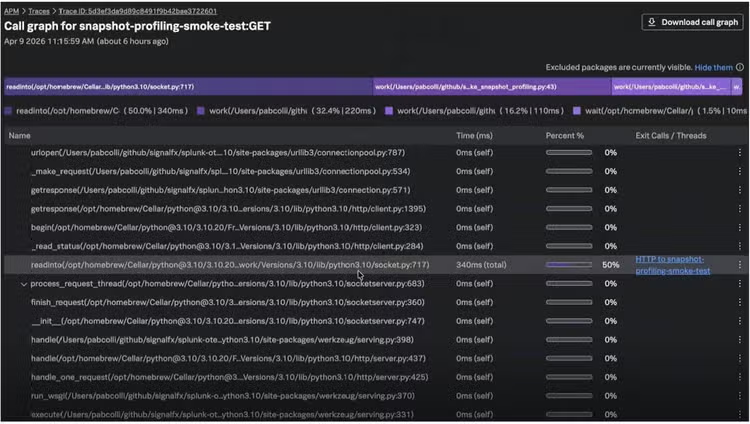
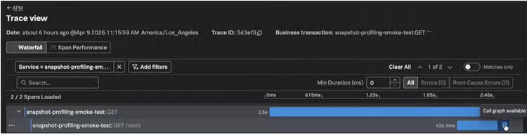
With Call Graph Profiling, the engineer can open the call graph associated with the span and inspect the methods executed during that request. The call graph preserves the parent-child hierarchy, so the team can see both the order of execution and the path that led to the expensive work. Exit calls and threads can link the investigation to the next call graph when execution crosses a boundary.

The summary bar highlights the methods with the greatest self-time—the method’s total duration minus the duration of its child methods. This distinction matters. A parent method might appear expensive because it waits for slow child calls, while a method with high self-time is spending that time in its own work. Splunk APM displays the top methods by self-time and lets investigators highlight the corresponding methods and table rows.

That gives operations and development teams a shared body of evidence:

• the business transaction affected
• the trace and span where latency occurred
• the method hierarchy involved
• the duration and percentage of call-stack time for each method; and
• the exit call or thread that continues the execution path.

Operations can identify a likely code owner with greater precision. Developers can begin with the actual execution path from the affected request rather than trying to reproduce the problem from a broad service-level symptom.

What Teams Can Find With a Call Graph

Call Graph Profiling can help uncover several common sources of poor application performance.

• High-latency methods: Method duration and percentage of call-stack time make unusually expensive methods easier to spot. The self-time summary helps distinguish methods doing substantial work themselves from methods whose duration comes primarily from descendants.
• Inefficient code paths: The method hierarchy can reveal redundant calls, avoidable repetition, or an unexpected execution branch. Seeing the sequence is particularly valuable when the code is correct functionally but inefficient operationally.
• Latency-intensive operations: A call graph can expose time spent in serialization, data transformation, computation, file access, or calls that leave the current execution context. Exit-call links help investigators continue following the work when the request moves elsewhere.
• Errors and exceptions: Code-level context can help connect a failing request to the relevant methods and lines of code, reducing the distance between observing an error and locating its likely cause.

A Practical Investigation Workflow:

Call Graph Profiling fits naturally into the way SRE, AppOps, ITOps, and development teams already troubleshoot applications.

1. Start with the user or business impact. Identify a slow service, endpoint, trace, or business transaction in Splunk APM.
2. Find the problematic span. Use the trace to determine where latency or an error appears in the distributed request.
3. Open the associated call graph. Move from span-level timing to the methods executed within the relevant request.
4. Review self-time first. Use the summary bar to identify methods contributing the most time directly.
5. Inspect the hierarchy. Expand child methods and follow the call path to understand how execution reached the hotspot.
6. Follow exit calls when needed. Continue to another call graph when the work crosses a service or thread boundary.
7. Share actionable evidence. Copy method names or download the call graph as JSON to support collaboration and deeper analysis.
8. Validate the fix. After optimizing the code, compare application latency and profiling evidence to confirm the outcome.

This workflow creates a cleaner division of labor without creating an information gap. Operations teams can isolate the symptom and likely hotspot; developers can focus immediately on why the method is slow and how to improve it.

Getting Started

Call Graph Profiling is available in Splunk Observability Cloud and requires Splunk APM, an AlwaysOn Profiling license, supported Splunk OpenTelemetry instrumentation, and a compatible Splunk Distribution of the OpenTelemetry Collector.

We support Java, .NET, Node.js, and Python.

The High-Level Setup Is Straightforward:

1. Confirm that your language runtime, Splunk OpenTelemetry instrumentation, and Collector meet the current prerequisites.
2. Instrument the application for Splunk APM so profiling data can be correlated with traces.
3. Enable Call Graph Profiling in the relevant language agent.
4. Verify that the profiling endpoint sends data to the Collector.
5. For Helm deployments, enable the shared logs and profiling pipeline in the Splunk OpenTelemetry Collector chart.
6. If you use a gateway deployment, ensure the agent-mode Collector receives profiling data locally and forwards it through a logs pipeline to the gateway.

Profiling adds runtime work, and higher-frequency sampling can increase CPU and memory usage. Test configuration changes in a staging environment, observe overhead, and tune selection probability and sampling intervals before rolling them into production. The default selection probability is 0.01, but you can adjust all the way up to 0.1. The setup guide and language-specific settings pages provide the latest configuration details.

Turn “The Service Is Slow” Into a Precise Next Step

The hardest part of troubleshooting is often not detecting a problem. It is moving from a broad signal to evidence specific enough for someone to act.

Call Graph Profiling shortens that journey. It connects distributed traces to the methods executed inside a request, exposes where time is spent, and preserves the hierarchy needed to understand why. Paired with AlwaysOn Profiling’s continuous view of application behavior, it gives teams both the wide-angle context and the request-level detail needed to improve performance.

For operations teams, that means a more precise handoff. For developers, it means less time reproducing symptoms and more time fixing the code that matters. For the business, it means a faster route from degraded experience to verified improvement.

Call graphs, as part of always on profiling, does requires Enterprise licensing. Learn more in the Splunk Call Graph Profiling documentation.